CV Study Notes - Classification I

Classification

The definition of classification is: categorizing a given set of data into classes

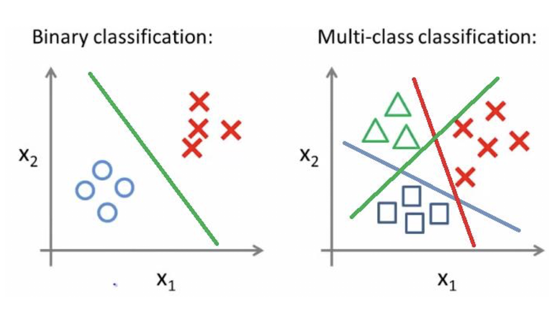
Example of classification(CAP5415 - Lecture 11 by L. Lazebnik)

This post will focus on the intuition of the classification algorithms including k-nearest neighbor and SVM. It is very interesting to learn the motivation and intuition behind each algorithm. No code or math will be involved in this post.

The Simplest Binary Classifier - Nearest Neighbor

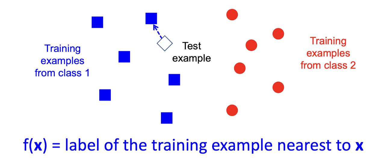
Illustration of nearest neighbor(CAP5415 - Lecture 11 by L. Lazebnik)

Given a new data point, calculate the distance between training samples, and take the class of the nearest sample.

The method is very simple and intuitive, however, it has some obvious disadvantages:

1. Not efficient: Has to calculate the distance for all the points
2. Sensitive for out-flyer

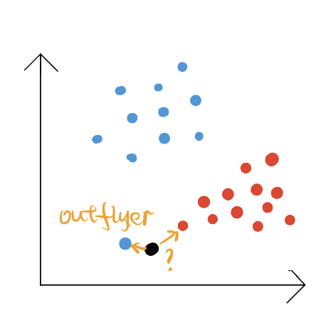
An example of out-flyer, the black dot is the new example that needs to be classified, the blue dot is the nearest point, however, the black dot should belong to the red class.

Solution?

How about we calculate multiple neighbors and determine the class by the mean of the label?

This lead to the K-nearest neighbor algorithm.

K-nearest Neighbor Classifier

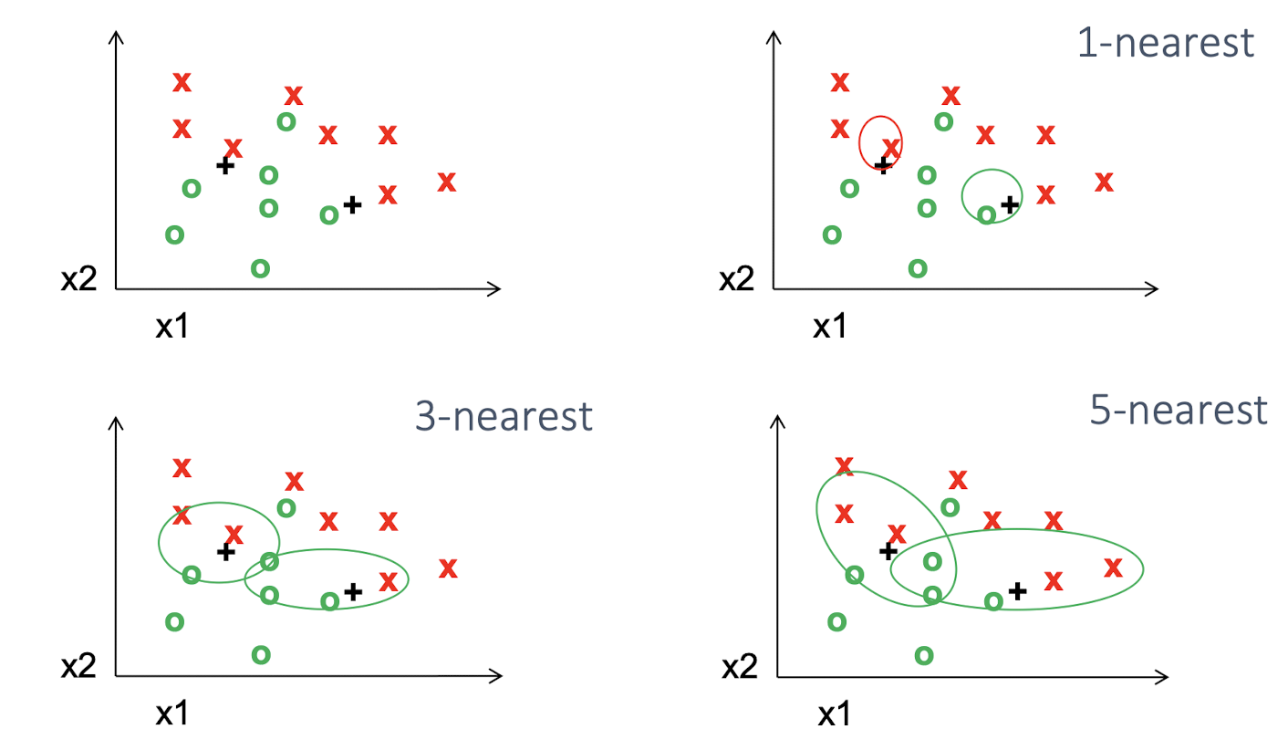
(CAP5415 - Lecture 11 by L. Lazebnik)

Instead of using the label of the nearest point, we can look around and consider the k-nearest neighbor. It’s simple and easy to implement but computationally expensive like the nearest neighbor classifier.

Linear Classifier

Motivation

The intuitive of classification is to find the boundary in the feature space of the samples.

Classify data set using a line for 2D data or a plane for 3D data. Take 2D as an example, it is to find a linear function to separate the classes. However, how can we determine which line to use?

More than one line can divide the data set(https://jakevdp.github.io/PythonDataScienceHandbook/05.07-support-vector-machines.html)

Maximum Margin Linear Classifier

To determine which line is the best separator, an intuitive idea is instead of drawing a zero-width line, we can draw the line with width, the wider the line is, the more precise the separation is.

The lines with width.(https://jakevdp.github.io/PythonDataScienceHandbook/05.07-support-vector-machines.html)

The maximum margin linear classifier is the linear classifier with the maximum margin. It is the simplest support vector machine, called linear support vector machine(LSVM). The line divided the two data sets with maximized width(margin). The training data points on the dashed line with the black circle are called support vectors. The distance from the support vector to the solid line is the margin. The model is determined by these support vectors.

Support Vectors(https://jakevdp.github.io/PythonDataScienceHandbook/05.07-support-vector-machines.html)

Issue: sometimes the data set is non-linearly separable, and the LSVM will perform poorly.

Non-linearly separable(https://jakevdp.github.io/PythonDataScienceHandbook/05.07-support-vector-machines.html)

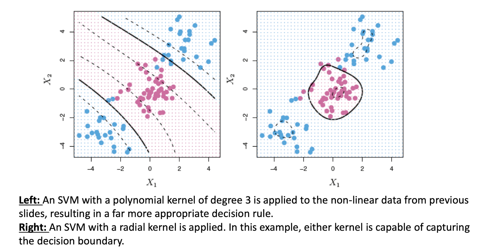
Kernel SVM

We can project the non-linearly separable data into higher-dimensional space defined by some function(kernel), and thereby the data can fit with a linear classifier.

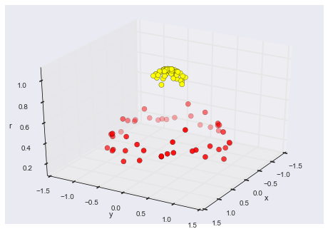
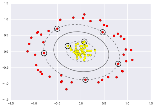
Here we can map the data using Radius Basis Function (RBF kernel) centered on the middle point to map the data from the non-separable 2D dimension to the separable 3D dimension.

Different kernel functions can be chosen to project the data to a higher dimension, but which kernel is best suitable for the data needed to be decided. Determining the center of the kernel is also difficult, but lucky for us, the built-in kernel trick process of SVM cover us.

Softening Margins

So far the data set in the example figures are all naturally separated. However, in the real case, the data points might be overlapping with each other, and there won’t a clear boundary between data points. Thus, another determining parameter for SVM is how soft the margin is which means allowing some of the points inside the margin if can get a better fit. If the margin is hard, the points can not get inside it. If it is soft, points can get inside the margin.

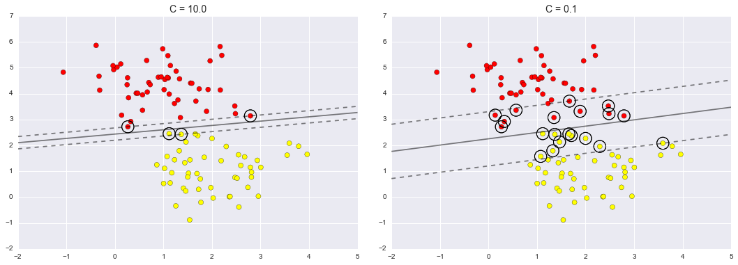
Left is the hard margin, Right is the soft margin.

References: https://jakevdp.github.io/PythonDataScienceHandbook/05.07-support-vector-machines.html https://www.crcv.ucf.edu/wp-content/uploads/2018/11/Lecture-11-Classification-I.pdf